Variational AI
  • Our Approach
  • Company
  • Team
  • Jobs
  • What’s New
  • Blog
  • Contact
  • How to drug a novel target in 500 molecules

    How to drug a novel target in 500 molecules

    Research conducted by the Variational AI team: Marshall Drew-Brook, Peter Guzzo, Ahmad Issa, Mehran Khodabandeh, Sara Omar, Jason Rolfe, and Ali Saberali.


    Searching through the space of synthesizable molecules to find an effective drug candidate is one of the most time-consuming and expensive steps of drug discovery. Once a protein mediating disease has been identified and some initial hits that weakly modulate the target have been found, this structure- and ligand-based information must bootstrap the hunt for a potent, selective, ADMET-compliant drug candidate. The associated hit-to-lead and lead optimization process takes multiple years and many millions of dollars (Paul, et al., 2010), driven by the large number of novel molecules that must be investigated to converge to a satisfactory drug candidate, and the cost of synthesizing each such molecule along the way.

    Artificial intelligence has the potential to accelerate hit-to-lead and lead optimization by reducing the number of novel compounds required to find a drug candidate. We show how active learning using Variational AI’s generative foundation model, Enki, can find extremely potent compounds for a novel target with data on only 500 molecules. Used in conjunction with absolute binding free energy (ABFE) calculations, Enki promises to identify potent, selective leads in mere weeks, and converge to a promising drug candidate in a few additional rounds of experimental synthesis and testing.To reconcile the disparity in generalization between QSAR and conventional machine learning tasks, we need to identify its cause. Three potential explanations present themselvesIn a succession of posts, we will explore each of these possibilities in turn, beginning with the first.

    Active learning is the AI embodiment of the design-make-test-analyze cycle

    Hit-to-lead and lead optimization are generally conducted via the design-make-test-analyze (DMTA) cycle. In each cycle (starting with “A”), the available experimental data is first analyzed. For instance, structure-activity relationships are characterized based upon series of molecules in which a single feature has been varied (e.g., ring size). New compounds are then designed by tuning molecular features that exhibit a consistent relationship with potency, selectivity, or other pharmacological properties, to their optimal values. These compounds are synthesized (made), tested, and used as the basis for further investigation.

    The DMTA cycle is an instance of active learning (or more precisely, Bayesian optimization), an AI paradigm for optimizing an objective (e.g., a weighted combination of potency, selectivity, and ADMET) by iteratively selecting points (e.g., molecules) for evaluation (Shahriari, et al., 2015). Bayesian optimization must balance exploration (e.g., of novel chemotypes) with exploitation (e.g., of previously identified potent scaffolds). The most effective Bayesian optimization algorithms explicitly model the uncertainty of predictions, and use the predicted uncertainty to maximize rigorous measures of search quality such as the expected improvement (Gómez-Bombarelli, et al., 2018; Griffiths & Hernández-Lobato, 2020). However, more heuristic approaches such as reinforcement learning (Olivecrona, et al., 2017), genetic algorithms (Jensen, 2019), and particle swarm optimization (Winter, et al., 2019) can also be used.

    Figure 1: The conventional DMTA cycle can be automated with Enki’s generative foundation model.

    Enki performs active learning via Bayesian optimization on a powerful, generative foundation model, pretrained on millions of potency data points across hundreds of targets. This allows it to find extremely potent ligands for a novel target, given target activity data on only 500 molecules, spread across five rounds DMTA/active learning. On each round of active learning, we fine-tune Enki on the available data for the novel target, and then search over the full space of synthesizable, drug-like molecules to find those that maximize the expected improvement of the predicted potency.

    Flexible architectures are almost unbeatable

    We evaluate Enki’s ability to optimize potency against three kinase targets of significant pharmacological interest: FGFR1, AURKA, and EGFR. While these are familiar drug targets, we render them novel for the purpose of this benchmark by removing all data on them, and all other targets with more than 65% homology, from the pretraining data. We then maximize pIC50 – 3*(1-QED), where QED is the quantitative estimate of drug-likeness (Bickerton, et al., 2012). The scale of the QED term is chosen to ensure that the best compounds in a 2.2M molecule screening set approximately satisfy Lipinski’s Rule of 5.

    Enki is initially fine-tuned on the potency of 100 randomly selected molecules against the optimization target. (The source library is the same used for high-throughput screening, described below.) In each of five succeeding rounds of active learning, Enki generates 100 molecules for potency evaluation that maximize the expected improvement of the predicted potency, and is fine-tuned to incorporate this data.

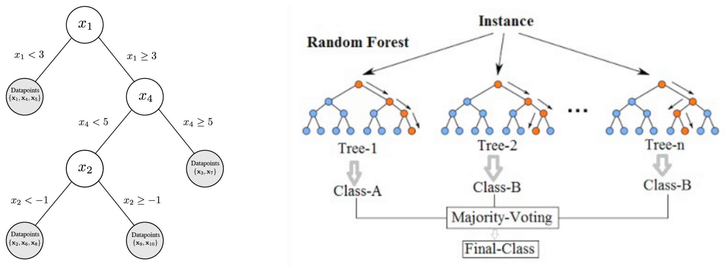
    We compare Enki to REINVENT (Olivecrona, et al., 2017; Loeffler, et al., 2024) and graph genetic algorithms (Graph GA; Jensen, 2019), the previous state-of-the-art in molecular optimization as determined by extensive benchmarking (Gao, et al., 2022; Nigam, et al., 2024). To adapt REINVENT and Graph GA to real-world lead optimization, where only a few novel molecules can be tested experimentally in each round of active learning, we equipped them with a QSAR model consisting of a random forest regressor operating on extended connectivity fingerprints (Dodds, et al., 2024; Nahal, et al., 2024). This architecture continues to achieve competitive performance for small molecule potency prediction (Cichońska, et al., 2021; Huang, et al., 2021; Luukkonen, et al., 2023; Stanley, et al., 2021; van Tilborg, et al., 2022).

    To facilitate fast and cost-effective benchmarking, we use molecular docking as a proxy for (not an approximation to) experimental potency. We treat docking scores as the true target endpoint, on the principle that if we can optimize docking scores using docking data, we should also be able to optimize experimental potencies using experimental data. As we have discussed in a previous post, molecular docking scores are a natural surrogate for experimental potencies because they are based upon the same geometry of pharmacophoric interactions that mediate experimental potency, are correlated with experimental potency, and are almost as difficult to predict as experimental potency. The docking scores are computed using Gnina’s CNNaffinity, a machine learning scoring function that is calibrated to pIC50 (McNutt, et al., 2021).

    We also compare to high-throughput screening by evaluating the true objective value for ~1.3M molecules that have previously been experimentally tested for kinase activity, ~0.4M molecules that have been tested for activity for other target classes, and ~0.5M molecules from the Enamine, WuXi, Otava, and Mcule make-on-demand sets. Half of the make-on-demand molecules were constrained to have a hinge binding scaffold, which is typical of kinase inhibitors. This library is biased towards compounds that are likely to bind to our targets, and thus represents a rigorous baseline for Enki.

    Flexible architectures are almost unbeatable

    The performance of active learning with Enki on three novel targets, compared to a high-throughput screen, is depicted in Figures 2 and 3. In all cases, the best of the Enki-optimized molecules is superior to any of the ~2M high-throughput screening molecules.

    The Enki-optimized molecules are novel relative to the 100 random molecules used to initialize active learning, as demonstrated in Figures 4, 5, and 6. We also evaluated synthesizability by performing retrosynthetic pathway prediction using Molecule.one. The distribution of the predicted number of synthetic steps is shown in Figure 7. For all three tasks, 90% of the Enki-optimized molecules were predicted to be synthesizable in fewer than ten steps.

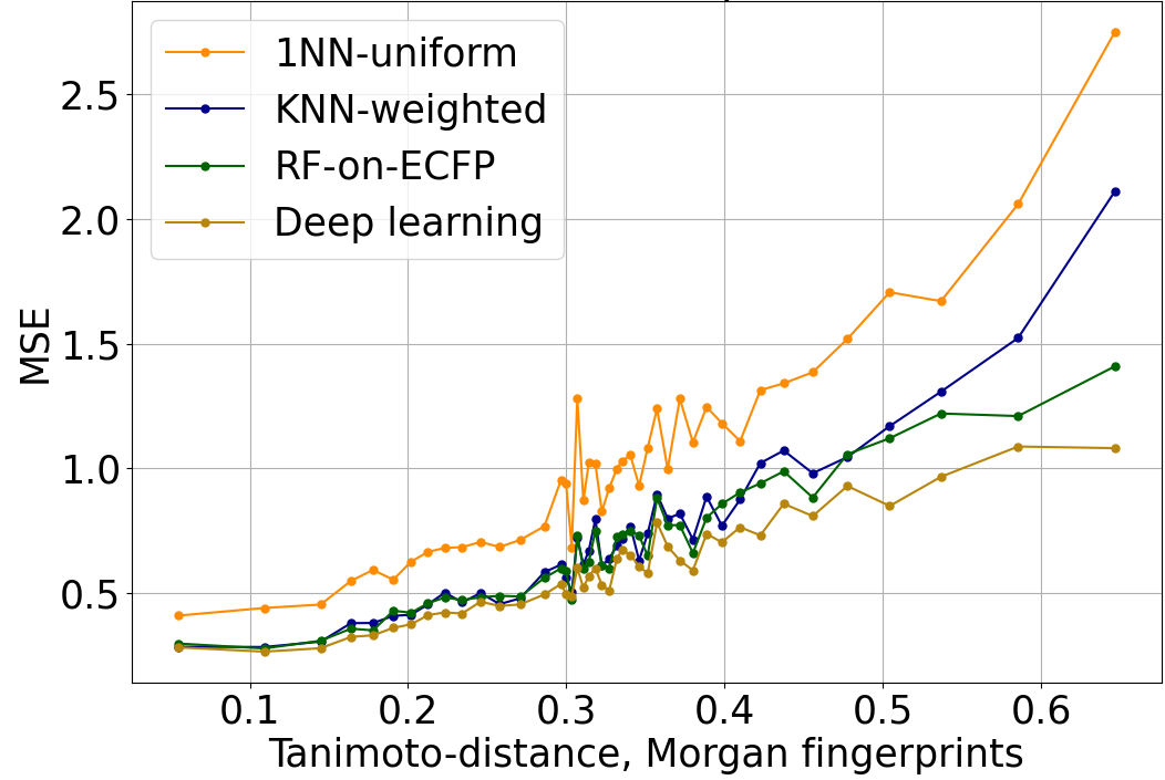
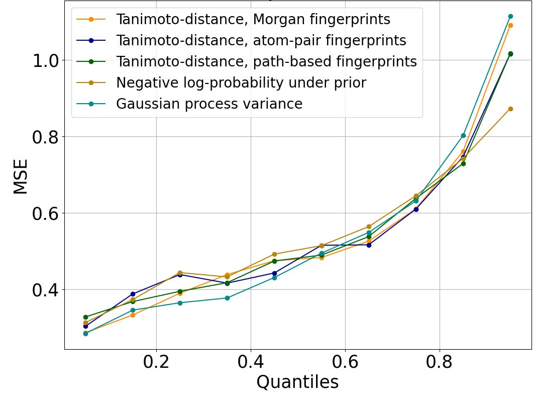
    We compared Enki, REINVENT, and Graph GA across five rounds of active learning, each comprising 100 molecules. As Figures 8 and 9 show, Enki produces molecules that better satisfy the optimization objective: pIC50 – 3*(1 – QED). These differences are highly statistically significant, with a large or very large effect size in all but one case (Table 1). Enki drives potency (CNNaffinity) to very high levels, significantly surpassing REINVENT and Graph GA as measured by both the mean over all 100 molecules in the last round of active learning, as well as when only considering the best molecules (Figure 10). In contrast, REINVENT and Graph GA over-optimize QED, driving it to excessive levels at the expense of potency (Figure 11). Enki’s effective potency optimization can be understood in terms of binding interactions in the docked poses (Figure 12).

    Figure 2: Distribution of the optimization objective values over high-throughput screening libraries, and Enki-optimized molecules from the fifth round of active learning, for the three benchmark tasks.

    Figure 3: Distribution of the optimization objective values over high-throughput screening libraries, and Enki-optimized molecules from the fifth round of active learning, for the three benchmark tasks, zoomed to highlight the best molecules.

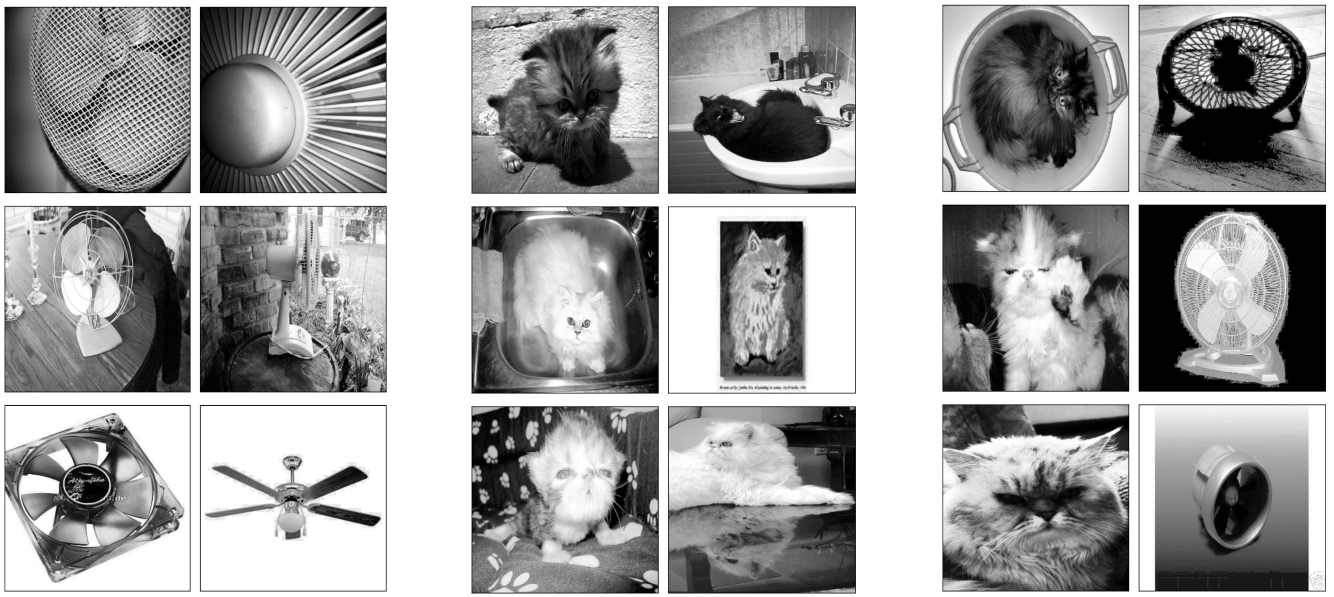
    Figure 4: Examples of Enki-optimized molecules from the fifth round of active learning for FGFR1 potency, along with the most similar molecules in the set of 100 molecules used to initialize optimization.

    Figure 5: Examples of Enki-optimized molecules from the fifth round of active learning for AURKA potency, along with the most similar molecules in the set of 100 molecules used to initialize optimization.

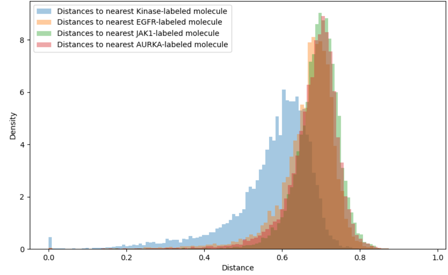
    Figure 6: Distribution of Tanimoto similarity of Enki-optimized molecules from the fifth round of active learning to the nearest molecule in the initial set of 100 molecules for the three benchmark tasks.

    Figure 7: Distribution of number of synthetic steps predicted by retrosynthetic pathway prediction for Enki-optimized molecules from the fifth round of active learning.

    Figure 8: Evolution of the optimization objective over five rounds of active learning using Enki, REINVENT, and Graph GA. Centerline, box, and whiskers indicate median, 25/75th percentile, 3/97th percentile, respectively. Additional points denote outliers beyond that range. For all targets, the round-5 Enki-optimized compounds are superior to those produced by REINVENT and Graph GA with p < 0.005 according to the Mann-Whitney U test.

    Figure 9: Distribution of the optimization objective for Enki, REINVENT, and Graph GA-optimized molecules from the fifth round of active learning. The mean of each distribution is denoted by a dotted line.

    Table 1: Statistical comparison of molecules from the fifth round of active learning produced by Enki, compared to REINVENT and Graph GA. P-values are computed using the Mann-Whitney U test and effect sizes are evaluated using Cohen’s d. d = 0.2 is considered a small effect size, d=0.5 is medium, d=0.8 is large, and 1.2 is very large.

    Figure 10: Distribution of the docking score (potency) for Enki, REINVENT, and Graph GA-optimized molecules from the fifth round of active learning. The mean of each distribution is denoted by a dotted line.

    Figure 11: Distribution of QED (quantitative estimate of drug-likeness) for Enki, REINVENT, and Graph GA-optimized molecules from the fifth round of active learning. The mean of each distribution is denoted by a dotted line.

    Figure 12: Evolution of ligand-protein interactions over multiple rounds of active learning with Enki.

    Efficient application of active learning in practice

    While active learning can be directly applied to experimental potency measurements, repeated rounds of unconstrained optimization over synthesizable, drug-like chemical space is time consuming and expensive. Even tractable de novo molecules can require months of effort and thousands of dollars to synthesize. Early rounds of active learning can be conducted more efficiently using computational approximations: first molecular docking, and then absolute binding free energy computations via free energy perturbations or thermodynamic integration.

    The results presented here suggest that active learning with Enki should converge to extremely potent ligands, as predicted by ABFE, with only a few hundred evaluations. Computation on this scale can be easily completed within a week on a moderately sized cluster. The compounds can then be synthesized and tested, and used to seed a few final rounds of active learning based upon experimental data.

    References

    Bickerton, G. R., Paolini, G. V., Besnard, J., Muresan, S., & Hopkins, A. L. (2012). Quantifying the chemical beauty of drugs. Nature chemistry, 4(2), 90-98.

    Cichońska, A., Ravikumar, B., Allaway, R. J., Wan, F., Park, S., Isayev, O., … & Challenge organizers. (2021). Crowdsourced mapping of unexplored target space of kinase inhibitors. Nature communications, 12(1), 3307.

    Dodds, M., Guo, J., Löhr, T., Tibo, A., Engkvist, O., & Janet, J. P. (2024). Sample efficient reinforcement learning with active learning for molecular design. Chemical Science, 15(11), 4146-4160.

    Gao, W., Fu, T., Sun, J., & Coley, C. (2022). Sample efficiency matters: a benchmark for practical molecular optimization. Advances in neural information processing systems, 35, 21342-21357.

    Gómez-Bombarelli, R., Wei, J. N., Duvenaud, D., Hernández-Lobato, J. M., Sánchez-Lengeling, B., Sheberla, D., … & Aspuru-Guzik, A. (2018). Automatic chemical design using a data-driven continuous representation of molecules. ACS central science, 4(2), 268-276.

    Griffiths, R. R., & Hernández-Lobato, J. M. (2020). Constrained Bayesian optimization for automatic chemical design using variational autoencoders. Chemical science, 11(2), 577-586.

    Huang, K., Fu, T., Gao, W., Zhao, Y., Roohani, Y., Leskovec, J., … & Zitnik, M. (2021). Therapeutics data commons: Machine learning datasets and tasks for drug discovery and development. arXiv preprint arXiv:2102.09548.

    Jensen, J. H. (2019). A graph-based genetic algorithm and generative model/Monte Carlo tree search for the exploration of chemical space. Chemical science, 10(12), 3567-3572.

    Loeffler, H. H., He, J., Tibo, A., Janet, J. P., Voronov, A., Mervin, L. H., & Engkvist, O. (2024). Reinvent 4: Modern AI–driven generative molecule design. Journal of Cheminformatics, 16(1), 20.

    Luukkonen, S., Meijer, E., Tricarico, G. A., Hofmans, J., Stouten, P. F., van Westen, G. J., & Lenselink, E. B. (2023). Large-scale modeling of sparse protein kinase activity data. Journal of Chemical Information and Modeling, 63(12), 3688-3696.

    McNutt, A. T., Francoeur, P., Aggarwal, R., Masuda, T., Meli, R., Ragoza, M., … & Koes, D. R. (2021). GNINA 1.0: molecular docking with deep learning. Journal of cheminformatics, 13(1), 43.

    Nahal, Y., Menke, J., Martinelli, J., Heinonen, M., Kabeshov, M., Janet, J. P., … & Kaski, S. (2024). Human-in-the-loop active learning for goal-oriented molecule generation. Journal of Cheminformatics, 16(1), 1-24.

    Nigam, A., Pollice, R., Tom, G., Jorner, K., Willes, J., Thiede, L., … & Aspuru-Guzik, A. (2024). Tartarus: A benchmarking platform for realistic and practical inverse molecular design. Advances in Neural Information Processing Systems, 36.

    Olivecrona, M., Blaschke, T., Engkvist, O., & Chen, H. (2017). Molecular de-novo design through deep reinforcement learning. Journal of cheminformatics, 9, 1-14.

    Paul, S. M., Mytelka, D. S., Dunwiddie, C. T., Persinger, C. C., Munos, B. H., Lindborg, S. R., & Schacht, A. L. (2010). How to improve R&D productivity: the pharmaceutical industry’s grand challenge. Nature reviews Drug discovery, 9(3), 203-214.

    Shahriari, B., Swersky, K., Wang, Z., Adams, R. P., & De Freitas, N. (2015). Taking the human out of the loop: A review of Bayesian optimization. Proceedings of the IEEE, 104(1), 148-175.

    Stanley, M., Bronskill, J. F., Maziarz, K., Misztela, H., Lanini, J., Segler, M., … & Brockschmidt, M. (2021, August). Fs-mol: A few-shot learning dataset of molecules. In Thirty-fifth Conference on Neural Information Processing Systems Datasets and Benchmarks Track (Round 2).

    van Tilborg, D., Alenicheva, A., & Grisoni, F. (2022). Exposing the limitations of molecular machine learning with activity cliffs. Journal of Chemical Information and Modeling, 62(23), 5938-5951.

    Winter, R., Montanari, F., Steffen, A., Briem, H., Noé, F., & Clevert, D. A. (2019). Efficient multi-objective molecular optimization in a continuous latent space. Chemical science, 10(34), 8016-8024.

    Jason Rolfe

    January 10, 2025
    Blog, Featured
  • Why is QSAR so far behind other forms of machine learning, and what can be done to close the gap?

    Why is QSAR so far behind other forms of machine learning, and what can be done to close the gap?

    The key feature of successful machine learning that is missing in QSAR

    In a previous post, we showed that the prediction error of QSAR (quantitative structure-activity relationship) models increases with the distance to the nearest element of the training set. This trend holds across a variety of machine learning algorithms and distance metrics. In contrast, prediction error is not correlated with distance to the training set on conventional ML (machine learning) tasks like image classification: modern deep learning algorithms are able to extrapolate far from their training data. 

    A favorable resolution of this apparent contradiction would have significant practical consequences. QSAR algorithms that generalize widely and accurately could efficiently identify new potent and selective molecules for difficult target product profiles, considerably reducing the time and expense of drug discovery.

    To reconcile the disparity in generalization between QSAR and conventional machine learning tasks, we need to identify its cause. Three potential explanations present themselves:

    1. Algorithms have been better aligned with conventional ML tasks,
    2. Better datasets have been brought to bear on standard ML tasks, or
    3. QSAR is intrinsically more difficult than typical ML tasks.

    In a succession of posts, we will explore each of these possibilities in turn, beginning with the first.

    QSAR algorithms do not capture the structure of ligand-protein binding

    Machine learning algorithms can correctly extrapolate some functions only because they are unable to extrapolate others (Wolpert & Macready, 1997). An algorithm that can represent every possible mapping from inputs to outputs equally well will memorize the training set, while producing arbitrary outputs on any other input. Correspondingly, ML algorithms generalize best when their architecture enforces the structure and regularities of the underlying problem domain. Such algorithms have difficulty representing irrelevant input-output mappings that violate the problem domain regularities, while easily capturing the true input-output mapping. Counterintuitively, recent state-of-the-art ML performance appears to be driven by increasingly flexible ML architectures, which are applicable across problem domains.

    This post will identify the key structural constraint that remains embedded in these ML algorithms: the consistent application of linear filters to local input patches. We will also show that the machine learning algorithms currently applied to small molecule potency prediction do not respect this structural constraint. The integration of local linear filters into QSAR (quantitative structure-activity relationship) models represents an untapped opportunity to improve potency prediction accuracy.

    ML architectures must be matched to the problem

    The visual domain exhibits significant structure and regularities. For instance, the semantic content of an image (e.g, whether or not an image contains a cat) is invariant to small shifts (e.g., vertical or horizontal), rotations, and scalings of the image. Critical features (e.g., edges and curves) in an image are composed of local, contiguous groups of pixels.

    Conventional neural networks, also called multi-layer perceptrons (MLPs), are not constrained to reflect the structure of images. Each unit (neuron) in an MLP computes a weighted sum of the units in the previous layer, followed by an activation function such as a rectified linear unit (ReLU; f(x) = max(0, x)) or a sigmoid (f(x) = 1/(1 + e-x)), as shown in Figure 1. Even the simplest one-hidden-layer MLP has unlimited power, and can represent any function mapping inputs (e.g., molecular structure) to outputs (e.g., log IC50 against a protein target), if the hidden layer is large enough (Hornik, et al., 1989).

    Figure 1: Architecture of a single unit in a multi-layer perceptron (MLP), and common activation functions. Many copies of this building block are repeated within and across layers. (Feng, et al., 2019)

    When an MLP is applied to a vision task, shifting an image up and to the right can completely transform the output, since the weights applied to each input pixel can change completely. On the other hand, if the pixels are rearranged before training (in a manner consistent between images), an MLP is not affected; it just permutes its weights in the same pattern. This lack of structure is evident in the filters (weights) learned by MLPs when applied to vision tasks. As shown in Figure 2, they do not contain any identifiable semantic features like edges, but rather look like high-frequency noise. Because MLPs do not embody enough structure of the problem domain, they generalize poorly (Bachman, et al., 2024).

    Figure 2: First layer linear filters from an unconstrained MLP (Bachman, et al., 2024), a convolutional neural network (Krizhevsky, et al., 2012), and a vision Transformer (patch embedding; Dosovitskiy, et al., 2020).

    The deep learning revolution was largely driven by the rise of convolutional neural networks (CNNs), which prominently embody the structure of the vision domain (Krizhevsky, et al., 2012). Convolutional networks apply a set of small pattern-matching filters (e.g., 3 pixels by 3 pixels) to every location in the image (Figure 3). In the early layers, these filters detect edges, as shown in Figure 2. Shifting the image up and to the right simply shifts the outputs of the filters. Eventually, filter outputs at nearby locations are pooled together, which virtually eliminates the effect of the shift.

    Figure 3: Architecture of a single unit of a convolutional neural network (CNN). Each unit applies a shared local, linear filter to a spatially-aligned patch of its input layer, followed by an activation function such as a ReLU. (Robson, 2017)

    Convolutional neural networks explicitly capture the invariance of semantic content to small shifts, as well as the fact that critical features (e.g., edges and curves) are composed of local, contiguous groups of pixels. They cannot easily produce classifications that change when the input is translated a few pixels to the right, or process images where the pixels have been arbitrarily rearranged, even if the permutation is consistent across all images. Correspondingly, CNNs achieve significantly better performance than MLPs on tasks like image classification (Bachman, et al., 2024).

    Devising new ML architectures to capture domain-specific features is difficult

    There is a long tradition of efforts to design new ML architectures that better capture the structure of the problem domain. Virtually none of these attempts have been successful. 

    In the visual domain, the semantic content of an image is also invariant to moderate changes in scaling (zoom), rotation (including out of plane), translation (shift), reflection (mirror image), lighting, and object pose. Architectures ranging from the scattering transform (invariant to rotation and scaling; Bruna & Mallat, 2013) to group equivariant CNNs (invariant to rotations and reflections; Cohen & Welling, 2016), geometric CNNs (invariant to pose; Bronstein, et al., 2017), and capsule networks (invariant to viewpoint and pose; Sabour, et al., 2017) have been developed that are invariant to these transformations. Despite their intuitive appeal, these approaches have not improved performance. The current state-of-the-art is based upon the vision Transformer, which eliminates even some of the explicit translational invariance of convolutional neural networks (Dosovitskiy, et al., 2020).

    In natural language, early work was dominated by parse trees. Recursive neural networks recapitulate the structure of parse trees by successively merging the representations of connected words and phrases (Socher, et al., 2010). This heavy, domain-specific structure was rendered unnecessary by the ascendance of recurrent neural networks (e.g. LSTMs and GRUs), which were inspired by the human ability to process words one at a time, in sequence (Hochreiter & Schmidhuber, 1997; Mikolov, et al., 2010; Cho, et al., 2014). They compute the summary of the first n words based only upon the preceding summary of the first n-1 words, combined with the nth word. Despite exhaustive explorations across the space of possible recurrent neural network architectures (e.g., Greff, et al., 2016), they have been supplanted by Transformers, which further weaken the architectural constraint by allowing the representation of each word to be directly influenced by every other word (Vaswani, et al., 2017). 

    Flexible architectures are almost unbeatable

    Most of the significant architectural advances in machine learning merely ensure that the learned function is as simple as possible. Examples include non-saturating activation functions (e.g., ReLU), dropout, normalization layers (e.g., batch norm), approximate second-order gradient descent (e.g., Adam) with learning rate decay and weight decay, residual connections, inverse bottleneck layers, label smoothing, attentional layers and gating (e.g, Transformers), and diffusion models. These architectural elements hold the learned function close to the identity transformation, which leaves the input unchanged, with deviations that are smooth or roughly linear.

    Other essential ML architectures capture only the most basic structure of the problem domain. Convolutional/recurrent networks enforce locality in and consistency across space/sequence, and have largely been supplanted by Transformers. Data augmentations (e.g., shifts, mixup; primarily applicable to visual data) enforce invariance to common distortions, including compositionality (adding a second object to an image doesn’t change the identity of the first object). Generative modeling (including masked auto-encoding, as in BERT) learns the joint distribution of the entire dataset, rather than the distribution of some variables (output) conditioned on other variables (input). 

    There are additional architectural elements that help the algorithm make maximal use of the training data: e.g., variational autoencoders, adversarial training, contrastive learning, and distillation. Other architectures are specific to specialized applications like equivariant graph neural networks and reinforcement learning. Nevertheless, this limited set of concepts is basically sufficient to understand how ChatGPT works its magic, and makes it clear that most advances in machine learning do not embed the detailed structure of the problem domain.

    The modest constraints imposed by domain-specific architectures are manifestations of Rich Sutton’s bitter lesson (Sutton, 2019):

    1) AI researchers have often tried to build knowledge into their agents, 2) this always helps in the short term, and is personally satisfying to the researcher, but 3) in the long run it plateaus and even inhibits further progress, and 4) breakthrough progress eventually arrives by an opposing approach based on scaling computation by search and learning.

    ML requires consistent local filters

    At the same time, some domain knowledge actually is required. All successful ML architectures apply a consistent set of local filters across the input. These filters extract key features in a manner robust to small perturbations or spurious correlations between distant inputs. In images, these filters must be able to detect local edges; in text, they must learn common n-grams. Without the domain knowledge implicit in local filters, performance collapses. 

    Convolutional neural networks explicitly apply local filters across the image (Figure 3). Vision Transformers construct the same filters implicitly through their self-attention mechanism (Cordonnier, et al., 2020; d’Ascoli, et al., 2021; for text Transformers, see Vig & Belinkov, 2019). The initial patch embedding in vision Transformers additionally applies explicit edge filters analogous to those of convolutional neural networks (Dosovitskiy, et al., 2020), as shown in Figure 2.

    MLP-Mixers eliminate even self-attention, and merely alternate between fully-connected layers across hidden units and spatial position, without significantly reducing performance (Tolstikhin, et al., 2021). These fully-connected layers implement non-local filters that cover the entire input, and are not consistent between different positions. However, MLP-Mixers begin with a patchification layer, which performs convolution (applies consistent local filters) with stride (offset between successive applications of the filter) equal to the filter size (Figure 4). The patchification layer differs from a conventional convolutional layer only in that there is no overlap between the regions to which the filters are applied.

    Figure 4: MLP-Mixers apply a patchification layer, which differs from a conventional convolution only in that the filter is shifted by a distance equal to its width between applications. (Bachman, et al., 2024)

    With its patchification layer, MLP-Mixer achieves a top-1 accuracy of 84.15% on ImageNet (a standard image classification dataset with 1.2M images spread across 1k categories; Tolstikhin, et al., 2021), comparable to vision Transformers (85.30% accuracy; Dosovitskiy, et al., 2020) and state-of-the-art convolutional networks (87.8% accuracy; Liu, et al., 2022) when all algorithms are pre-trained on ImageNet-21k. Even if communication is not allowed between the patches before the final classification, patchification during the initial embedding facilitates reasonable performance: 56.5% top-1 accuracy on ImageNet even without extra pre-training data (Touvron, et al., 2021). If the patchification layer is removed, eliminating all consistent local filtering, the performance of the resulting MLP collapses to 31.7% (no pre-training; Bachman, et al., 2024). MLP accuracy decays further to 8.7% without data augmentation, such as random shifts and flips, which implicitly enforce the invariance captured explicitly by convolution/patchification.

    Convolution or patchification layers, which apply consistent local linear filters, are the key driver of prediction accuracy. A variety of different strategies for passing information between spatial positions yield similar performance, so long as local linear filtering is also performed (Liu, et al., 2021; Tolstikhin, et al., 2021; Touvron, et al., 2021; Yu, et al., 2022).

    Current ML architectures cannot produce consistent local filters for small molecules

    It is difficult to construct an analogous filtering or patchification operation on molecular graphs. For local filters to be useful, the precise relationship and alignment between nearby regions must be evaluated. In the vision domain, filter alignment captures the difference between two nearby edges that form a single line and orthogonal edges that belong to different shapes. Computer vision algorithms such as convolutional neural networks and vision Transformers can easily evaluate alignment between rotationally asymmetric local filters (e.g., edge detectors) because the filters are defined relative to a global orientation: “up” is consistent between patches and images. 

    Molecular graphs do not have a privileged global orientation against which rotationally asymmetric local filters can be aligned. Imposing an arbitrary global orientation would require the algorithm to separately learn every possible orientation, rather than embodying invariance to global orientation in the consistency of the local filters. In the image domain, this would be analogous to using unconstrained MLPs without convolution or patchification layers (eliminating the consistency of local filters), and instead applying random shifts to every image to train the unconstrained MLP to be invariant to these transformations. As we saw above, removing this explicit embodiment of shift-invariance significantly hurts performance. 

    A naive extension of patches to molecular graphs might uniquely encode each radius-n sub-graph. Extended connectivity fingerprints (ECFPs) approximate this process, but hash to a smaller number of bits, so the same representation is assigned to multiple unrelated patches (Rogers & Hahn, 2010). ECFPs are approximated in turn by graph convolutional networks, to the extent that the per-node feedforward layer(s) approximate a hash function (Xu, et al., 2019). This patchification is radially symmetric, and does not align representations between patches. Since even similar patches (radius-n sub-graphs) have maximally distant representations in these approaches, they do not facilitate generalization. In contrast, in state-of-the-art ML algorithms, image patches are processed by aligned linear filters, for which the output changes smoothly as the input is altered. 

    Many modern QSAR algorithms are based upon SMILES strings, which cut the rings of a molecule to form a tree, and then walk through the tree, reading out atoms and bonds as they are encountered (Chithrananda, et al., 2020; Ross, et al., 2022). There are many valid SMILES strings that equally represent a single molecule. Each such SMILES string highlights some bonds, by presenting the bonded atoms consecutively; and deemphasizes others, for which the atoms are distant in the SMILES string. In any single SMILES string, some local fragments of the molecule will be split up across faraway sections of the SMILES string, and thus not subject to processing by local filters on the SMILES string (Figure 5). 

    Figure 5: Multiple SMILES strings of the same molecule, with the traversal path of the SMILES string overlaid on the molecular graph. Each SMILES string represents a different subset of bonded atoms using consecutive tokens.

    Graph neural networks (Kipf & Welling, 2016; Veličković, et al., 2018; Xu, et al., 2019) and graph Transformers (Ying, et al., 2021; Dwivedi, et al., 2023) are often hailed as the obvious architectures for molecular property prediction (Atz, et al., 2021; Müller, et al., 2023), but they do not consistently surpass even simple architectures like random forests on extended connectivity fingerprints for experimental activity prediction (Cichońska, et al., 2021; Huang, et al., 2021; Deng, et al., 2022; Luukkonen, et al., 2023). Graph neural networks effectively apply a filter that takes the average of the connected nodes. In the visual domain, this would correspond to only using the filter 

    which averages nearby pixels and smooths away fine details (Figure 6). This extremely limited filter only achieves good performance in the visual domain when used in conjunction with multiple patchification layers, which apply complicated, consistent local filters (Yu, et al., 2022). Without separate patchification, graph neural networks constitute low-pass filters, and suffer from the over-smoothing problem: the representations of all nodes converge to a common value exponentially quickly in the number of layers (Oono & Suzuki, 2020; Rusch, et al., 2023). After a few layers, all but one node can be safely ignored, since the nodes are all identical. Attentional mechanisms do not resolve this limitation (Wu, et al., 2024). 

    Figure 6: A 3×3 low-pass filter only smooths an image, and does not identify important features. Graph neural networks effectively apply such a low-pass filter, rather than using trained filters as in a traditional convolutional neural network.

     Moreover, graph neural networks are structurally incapable of distinguishing between pairs of molecules with significant differences, such as those in Figure 7 (Xu, et al., 2019). They cannot even count the number of each functional group present in a molecule (Chen, et al., 2020), a task which should be easily solvable using consistent local filters (by constructing a filter for each functional group, and summing the filtered outputs).

    Figure 7: Graph neural networks, including Graph Isomorphism Networks (GIN; Xu, et al., 2019) and Graph Attention Networks (GAT; Veličković, et al., 2018), are unable to distinguish between these two molecules. They produce identical predictions, regardless of how the network is trained. The confusion arises because there is a correspondence between the atoms (indicated by matching colors in the figure), such that the neighborhoods of corresponding atoms also correspond. For example, in both molecules, a blue carbon is connected to a blue carbon, a magenta carbon, and a green fragment.

    Transformers break their input into discrete tokens, which are all processed in the same way. In text, each word (or word part) constitutes a distinct token. On images, tokens typically comprise large (e.g., 16 x 16) pixel patches (Dosovitskiy, et al., 2020). Since tokens are processed uniformly, the position of each token within the text or image must be captured in the token’s embedding (the vector representation assigned to the token). This is achieved via a positional encoding, which is added to the encoding of the content before the first Transformer layer. The traditional positional encoding is a set of sinusoids, which captures the relative distance between each pair of tokens along the key axes (sequence for text; x and y axes for images). 

    Corresponding positional encodings cannot be easily constructed for molecular graphs, since they lack unique axes that are consistent between different molecules. (There is no well-defined “up” direction.) The most common graph positional encodings include those based on the path distance (the number of bonds between two atoms, using either shortest paths or random walks; Ying, et al., 2021; Dwivedi, et al., 2021), or the eigenvectors of the graph Laplacian (the vibrational modes if the atoms were point masses and the bonds were springs; Dwivedi, et al., 2023). 

    A positional encoding based upon path distances can only construct rotationally symmetric filters. On an image (connecting each pair of adjacent pixels, resulting in a square grid), such a positional encoding cannot produce the edge filters required for image classification. 

    The eigenvectors of the graph Laplacian do not have a well-defined sign: they define axes, but do not distinguish between the two directions along each axis (Huang, et al., 2023). Moreover, they do not distinguish between rotations amongst eigenvectors with repeated eigenvalues, and can be unstable to even small changes in the graph (Figure 8; Wang, et al., 2022). Between dissimilar molecular graphs, there is no obvious relationship amongst corresponding eigenvectors. As a result, the eigenvectors of the graph Laplacian do not define consistent axes between different molecular graphs. 

    Figure 8: Corresponding eigenvectors (ordered by eigenvalue) of similar and dissimilar molecules are visualized on the molecular graphs using a cold-to-hot color scale. Eigenvector 6 is mostly consistent between the similar molecules. The two other eigenvectors are reordered or significantly different. Eigenvectors have an even weaker correspondence between dissimilar molecules.

    Some early efforts applied 3D convolutional neural networks to the voxelization of 3D molecular poses (Wallach, et al., 2015; Ragoza, et al., 2017; Jiménez, et al., 2018; Stepniewska-Dziubinska, et al., 2018). While they do explicitly utilize consistent local filters, and are robust to shifts, 3D CNNs have no intrinsic invariance to rotations. The set of rotations to which the network must be robust is much larger than in the case of computer vision, since there is no global “up” direction to which inputs can be aligned. Computational requirements and voxel sparsity increase cubically with the grid resolution, so such 3D CNNs have typically used coarse grids, rendering them blind to perturbations as large as 0.5 or 1 Å. Moreover, a single conformer must be chosen, which may bear little resemblance to the bound pose of the ligand to any particular target. Because of these difficulties, few modern QSAR algorithms are based on 3D CNNs (Wallach, et al., 2024).

    Conclusion

    The success of machine learning in domains like vision and natural language depends upon the consistent application of local linear filters across the input. Unfortunately, standard QSAR approaches based upon molecular fingerprints, SMILES strings, graph neural networks, and graph Transformers fail to perform a corresponding filtering operation on molecular graphs. The absence of consistent local filters may explain the relative poor performance of powerful deep learning algorithms on QSAR tasks. Efforts should be directed towards developing techniques to apply consistent local filters to molecular graphs.

    Acknowledgements

    Thanks to Mehran Khodabandeh for making most of the figures in this post.

    References

    Atz, K., Grisoni, F., & Schneider, G. (2021). Geometric deep learning on molecular representations. Nature Machine Intelligence, 3(12), 1023-1032.

    Bachmann, G., Anagnostidis, S., & Hofmann, T. (2024). Scaling mlps: A tale of inductive bias. Advances in Neural Information Processing Systems, 36.

    Bronstein, M. M., Bruna, J., LeCun, Y., Szlam, A., & Vandergheynst, P. (2017). Geometric deep learning: going beyond euclidean data. IEEE Signal Processing Magazine, 34(4), 18-42.

    Bruna, J., & Mallat, S. (2013). Invariant scattering convolution networks. IEEE transactions on pattern analysis and machine intelligence, 35(8), 1872-1886.

    Chen, Z., Chen, L., Villar, S., & Bruna, J. (2020). Can graph neural networks count substructures?. Advances in neural information processing systems, 33, 10383-10395.

    Chithrananda, S., Grand, G., & Ramsundar, B. (2020). ChemBERTa: large-scale self-supervised pretraining for molecular property prediction. arXiv preprint arXiv:2010.09885.

    Cho, K., van Merriënboer, B., Gu̇lçehre, Ç., Bahdanau, D., Bougares, F., Schwenk, H., & Bengio, Y. (2014, October). Learning Phrase Representations using RNN Encoder–Decoder for Statistical Machine Translation. In Proceedings of the 2014 Conference on Empirical Methods in Natural Language Processing (EMNLP) (pp. 1724-1734).

    Cichońska, A., Ravikumar, B., Allaway, R. J., Wan, F., Park, S., Isayev, O., … & Challenge organizers. (2021). Crowdsourced mapping of unexplored target space of kinase inhibitors. Nature communications, 12(1), 3307.

    Cohen, T., & Welling, M. (2016, June). Group equivariant convolutional networks. In International conference on machine learning (pp. 2990-2999). PMLR.

    Cordonnier, J. B., Loukas, A., & Jaggi, M. (2019). On the relationship between self-attention and convolutional layers. arXiv preprint arXiv:1911.03584.

    d’Ascoli, S., Touvron, H., Leavitt, M. L., Morcos, A. S., Biroli, G., & Sagun, L. (2021, July). Convit: Improving vision transformers with soft convolutional inductive biases. In International conference on machine learning (pp. 2286-2296). PMLR.

    Deng, J., Yang, Z., Wang, H., Ojima, I., Samaras, D., & Wang, F. (2023). A systematic study of key elements underlying molecular property prediction. Nature Communications, 14(1), 6395.

    Dosovitskiy, A., Beyer, L., Kolesnikov, A., Weissenborn, D., Zhai, X., Unterthiner, T., … & Houlsby, N. (2020). An image is worth 16×16 words: Transformers for image recognition at scale. arXiv preprint arXiv:2010.11929.

    Dwivedi, V. P., Luu, A. T., Laurent, T., Bengio, Y., & Bresson, X. (2021). Graph neural networks with learnable structural and positional representations. arXiv preprint arXiv:2110.07875.

    Dwivedi, V. P., Joshi, C. K., Luu, A. T., Laurent, T., Bengio, Y., & Bresson, X. (2023). Benchmarking graph neural networks. Journal of Machine Learning Research, 24(43), 1-48.

    Feng, J., He, X., Teng, Q., Ren, C., Chen, H., & Li, Y. (2019). Reconstruction of porous media from extremely limited information using conditional generative adversarial networks. Physical Review E, 100(3), 033308.

    Greff, K., Srivastava, R. K., Koutník, J., Steunebrink, B. R., & Schmidhuber, J. (2016). LSTM: A search space odyssey. IEEE transactions on neural networks and learning systems, 28(10), 2222-2232.

    Hochreiter, S., & Schmidhuber, J. (1997). Long short-term memory. Neural computation, 9(8), 1735-1780.

    Hornik, K., Stinchcombe, M., & White, H. (1989). Multilayer feedforward networks are universal approximators. Neural networks, 2(5), 359-366.

    Huang, K., Fu, T., Gao, W., Zhao, Y., Roohani, Y., Leskovec, J., … & Zitnik, M. (2021). Therapeutics data commons: Machine learning datasets and tasks for drug discovery and development. arXiv preprint arXiv:2102.09548.

    Huang, Y., Lu, W., Robinson, J., Yang, Y., Zhang, M., Jegelka, S., & Li, P. (2023). On the stability of expressive positional encodings for graph neural networks. arXiv preprint arXiv:2310.02579.

    Jiménez, J., Skalic, M., Martinez-Rosell, G., & De Fabritiis, G. (2018). K deep: protein–ligand absolute binding affinity prediction via 3d-convolutional neural networks. Journal of chemical information and modeling, 58(2), 287-296.

    Kipf, T. N., & Welling, M. (2016). Semi-supervised classification with graph convolutional networks. arXiv preprint arXiv:1609.02907.

    Krizhevsky, A., Sutskever, I., & Hinton, G. E. (2012). Imagenet classification with deep convolutional neural networks. Advances in neural information processing systems, 25.

    Liu, H., Dai, Z., So, D., & Le, Q. V. (2021). Pay attention to mlps. Advances in neural information processing systems, 34, 9204-9215.

    Liu, Z., Mao, H., Wu, C. Y., Feichtenhofer, C., Darrell, T., & Xie, S. (2022). A convnet for the 2020s. In Proceedings of the IEEE/CVF conference on computer vision and pattern recognition (pp. 11976-11986).

    Luukkonen, S., Meijer, E., Tricarico, G. A., Hofmans, J., Stouten, P. F., van Westen, G. J., & Lenselink, E. B. (2023). Large-scale modeling of sparse protein kinase activity data. Journal of Chemical Information and Modeling, 63(12), 3688-3696.

    Mikolov, T., Karafiát, M., Burget, L., Cernocký, J., & Khudanpur, S. (2010, September). Recurrent neural network based language model. In Interspeech (Vol. 2, No. 3, pp. 1045-1048).

    Müller, L., Galkin, M., Morris, C., & Rampášek, L. (2023). Attending to graph transformers. arXiv preprint arXiv:2302.04181.

    Oono, K., & Suzuki, T. (2020). Graph neural networks exponentially lose expressive power for node classification. arXiv preprint arXiv:1905.10947.

    Ragoza, M., Hochuli, J., Idrobo, E., Sunseri, J., & Koes, D. R. (2017). Protein–ligand scoring with convolutional neural networks. Journal of chemical information and modeling, 57(4), 942-957.

    Robson, R. (2017). Convolutional neural networks – Basics. MLNotebook. https://mlnotebook.github.io/post/CNN1/

    Rogers, D., & Hahn, M. (2010). Extended-connectivity fingerprints. Journal of chemical information and modeling, 50(5), 742-754.

    Ross, J., Belgodere, B., Chenthamarakshan, V., Padhi, I., Mroueh, Y., & Das, P. (2022). Large-scale chemical language representations capture molecular structure and properties. Nature Machine Intelligence, 4(12), 1256-1264.

    Rusch, T. K., Bronstein, M. M., & Mishra, S. (2023). A survey on oversmoothing in graph neural networks. arXiv preprint arXiv:2303.10993.

    Socher, R., Manning, C. D., & Ng, A. Y. (2010, December). Learning continuous phrase representations and syntactic parsing with recursive neural networks. In Proceedings of the NIPS-2010 deep learning and unsupervised feature learning workshop (Vol. 2010, pp. 1-9).

    Stepniewska-Dziubinska, M. M., Zielenkiewicz, P., & Siedlecki, P. (2018). Development and evaluation of a deep learning model for protein–ligand binding affinity prediction. Bioinformatics, 34(21), 3666-3674.

    Sutton, R. (2019). The bitter lesson. http://www.incompleteideas.net/IncIdeas/BitterLesson.html

    Tolstikhin, I. O., Houlsby, N., Kolesnikov, A., Beyer, L., Zhai, X., Unterthiner, T., … & Dosovitskiy, A. (2021). Mlp-mixer: An all-mlp architecture for vision. Advances in neural information processing systems, 34, 24261-24272.

    Touvron, H., Bojanowski, P., Caron, M., Cord, M., El-Nouby, A., Grave, E., … & Jégou, H. (2022). Resmlp: Feedforward networks for image classification with data-efficient training. IEEE Transactions on Pattern Analysis and Machine Intelligence, 45(4), 5314-5321.

    Vaswani, A., Shazeer, N., Parmar, N., Uszkoreit, J., Jones, L., Gomez, A. N., … & Polosukhin, I. (2017). Attention is all you need. Advances in neural information processing systems, 30.

    Veličković, P., Cucurull, G., Casanova, A., Romero, A., Lio, P., & Bengio, Y. (2018). Graph attention networks. arXiv preprint arXiv:1710.10903.

    Vig, J., & Belinkov, Y. (2019). Analyzing the structure of attention in a transformer language model. arXiv preprint arXiv:1906.04284.

    Wallach, I., Dzamba, M., & Heifets, A. (2015). AtomNet: a deep convolutional neural network for bioactivity prediction in structure-based drug discovery. arXiv preprint arXiv:1510.02855.

    Wallach & The Atomwise AIMS Program. (2024). AI is a viable alternative to high throughput screening: a 318-target study. Sci Rep 14, 7526. 

    Wang, H., Yin, H., Zhang, M., & Li, P. (2022). Equivariant and stable positional encoding for more powerful graph neural networks. arXiv preprint arXiv:2203.00199.

    Wu, X., Ajorlou, A., Wu, Z., & Jadbabaie, A. (2024). Demystifying oversmoothing in attention-based graph neural networks. Advances in Neural Information Processing Systems, 36.

    Xu, K., Hu, W., Leskovec, J., & Jegelka, S. (2019). How powerful are graph neural networks?. arXiv preprint arXiv:1810.00826.

    Ying, C., Cai, T., Luo, S., Zheng, S., Ke, G., He, D., … & Liu, T. Y. (2021). Do transformers really perform badly for graph representation?. Advances in neural information processing systems, 34, 28877-28888.

    Yu, W., Luo, M., Zhou, P., Si, C., Zhou, Y., Wang, X., … & Yan, S. (2022). Metaformer is actually what you need for vision. In Proceedings of the IEEE/CVF conference on computer vision and pattern recognition (pp. 10819-10829).

    Jason Rolfe

    September 14, 2024
    Blog
  • 100 AI-generated molecules are worth a 1,000,000 molecule high-throughput screen

    100 AI-generated molecules are worth a 1,000,000 molecule high-throughput screen

    The agony and the ecstasy of generative AI for small molecule drug discovery

    Research conducted by the Variational AI team: Marawan Ahmed, Marshall Drew-Brook, Peter Guzzo, Ahmad Issa, Mehran Khodabandeh, Jason Rolfe, and Ali Saberali.

    Drug discovery requires the identification of novel molecules that efficiently reach their site of action in the body, potently modulate a biological target that mediates disease, avoid interfering with other critical processes in the body, and are safely eliminated after an appropriate interval. The staggering difficulty of this task is reflected in the approximately 10 years and $2 billion required to develop a new drug (DiMasi, et al., 2016).

    Artificial intelligence has been touted as a panacea for every step of this process, from synthesizing the biomedical literature into hypothetical drug targets (Savage, 2023), to recruiting patients for clinical trials (Hutson, 2024). Over $59 billion has been invested in companies purporting to use AI to discover new drugs. The successes claimed by these companies are often hyperbolic, but the cost of rigorous testing makes it difficult to separate fact from fiction. 

    In this post, we summarize the current state of small molecule hit discovery, propose an unbiased benchmark for generative AI algorithms, and show that 100 molecules created by Variational AI’s algorithm, Enki, are as effective as a high-throughput screen over 1,000,000 molecules.

    Conventional approaches to hit discovery 

    A few drugs, including penicillin, quinine, and benzodiazepines, were stumbled upon by luck and vigilance. Others were the result of small modifications of existing drugs, designed to escape patents (Brown, 2023). When serendipity fails and incremental improvements are insufficient, rational drug discovery offers an alternative. 

    Rational drug discovery depends upon the identification of a biological target, generally a protein, for which inhibition, activation, or some other modulation is believed to have a beneficial medical effect. Once the target is chosen, rational discovery generally commences by evaluating a large, fixed set of molecules for potent hits against the target. This evaluation can be conducted experimentally, using biochemical or cellular assays, or virtually, using molecular docking or a QSAR (quantitative structure-activity relationship) model.

    In an experimental high-throughput screen, tens of thousands to a few million drug-like but target-independent compounds, predeposited on 96, 384, or 1536-well plates, are tested for activity against the target at a single concentration. These measurements are subject to noise due to the formation of colloidal aggregates, direct assay interference, compound degradation or contamination, reactivity, and the like (Aldrich, et al., 2017). Correspondingly, most of the apparent hits in primary screens are usually revealed to be false positives by more accurate confirmatory and counter-screens (Shun, et al., 2011), and the median hit rate is significantly less than 1% (Jacoby, et al., 2005; Lloyd, 2020; Schuffenhauer, et al., 2005). The size of such screens can be scaled to a few billion compounds using DNA-encoded libraries (DELs), at the cost of restrictive chemistries and assays, and potential interference from the DNA labeling process (Peterson & Liu, 2023). 

    Virtual high-throughput screening can also expand the screening libraries to a few billion compounds by relying upon molecular docking or QSAR models in place of experimental potency assays (Gorgulla, et al., 2020). In a few such extremely large virtual screens, rates of 10-40% have been reported (Bender, et al., 2021), but hit rates around 10% are more typical (Damm-Ganamet, et al., 2019; Slater & Kontoyianni, 2019; Zhu, et al, 2013). The success of virtual screening can depend upon the virtuosity of the docking protocol design and manual hit picking, and the tractability of the target (Zhu, et al., 2022). Recent experiments have shown that as the size of the virtual screening library increases to one billion molecules, almost all top-ranked molecules are artifacts of the scoring function used by molecular docking (Lyu, et al., 2023).

    As a conspicuous example of these difficulties, tens of thousands of papers applied virtual screening to SARS-CoV-2 over the course of the COVID-19 pandemic, but few developable leads resulted from this extensive effort (Gentile, et al., 2023; Macip, et al, 2021).  Similarly, in the recent CACHE challenge to find molecules that bind to the WD40 domain of LRRK2 (a previously undrugged target), none of the 1,955 tested compounds achieved Kd < 10μM (Ackloo, et al., 2022; results of CACHE challenge #1). Across 318 virtual high-through screening campaigns against challenging targets, Atomwise only observed reliable experimental activity on ~3% of their virtual hits, with some of these hits as weak as 865 μM, and no hits at all identified for 26% of the targets (Wallach, et al., 2024).

    Machine learning enables many of the largest virtual screens. An ML regressor is trained on the docking scores of a small subset of the virtual molecule library, and then used as a low-cost approximation to triage the remaining compounds (Gentile, et al., 2020). The inaccuracy of this triage can be reduced by applying multiple active learning cycles, in which the machine learning regressor is fine-tuned on the true docking scores of the molecules selected in the previous round of triaging. However, accuracy is still bounded by that of molecular docking. 

    Even the largest libraries used in DELs and ML-augmented virtual screens cover approximately 0% of the 1023 to 1060 synthesizable, drug-like molecules that are believed to exist (Ertl, 2023; Polishchuk, et al., 2013; Bohacek, et al, 1996). Perhaps more importantly, these screens only search for potency to a single on-target. Discovering potent hits is actually the easiest step in drug discovery, historically taking around one year and $1M in a large pharma environment (Paul, et al., 2010). Engineering selectivity and ADMET (absorption, distribution, metabolism, excretion, and toxicity) constraints into such hits is a challenge left for hit-to-lead and lead optimization, a significantly more difficult task requiring 3.5 years and $12.5M. Even then, this process may overlook the best drug candidates, with exceptional selectivity and ADMET, which may lie in regions of chemical space that are distant from the compounds with the highest potency to the primary target. 

    Generative AI promises to revolutionize hit discovery by efficiently searching over a significant fraction of the 1060 synthesizable, drug-like molecules, and jointly optimizing for potency, selectivity, ADME, and toxicity. However, promise is not the same thing as performance, and the field is rife with unsubstantiated hype. 

    The agony of benchmarking generative AI for hit discovery

    The synthesis and experimental testing of an AI-generated molecule with a novel chemotype requires thousands of dollars and months of effort. As a result, many groups enlist computational and medicinal chemists to choose only a handful of molecules for synthesis and experimental evaluation, out of the tens of thousands of candidates constructed by their generative AI. Zhavoronkov, et al. (2019) selected 6 compounds for synthesis out of 30,000 produced by their generative AI algorithm; Tan, et al. (2021) selected 2 out of 19,929; Yoshimori, et al. (2021) selected 9 out of 570,542; Jang, et al. (2022) selected 1 out of 10,416; Li, et al (2022) selected 8 out of 79,323; Ren, et al. (2023) selected 7 out of 8,918; and Chenthamarakshan, et al. (2023) selected 4 out of 875,000. 

    It is unclear what proportion of the real work is being done by human experts in the process of selecting 0.01% of the AI-generated molecules. Indeed, the AI algorithm itself may almost exclusively produce inactive, non-selective, unsynthesizable, or non-drug-like molecules (Gao & Coley, 2020). And since only one algorithm is tested in each of these efforts, it is impossible to compare the AI algorithms to each other, or to conventional techniques like high-throughput screening. 

    To conduct an unbiased, statistically meaningful evaluation of generative AI methods, hundreds of molecules must be selected by each AI algorithm for a common task, without human assistance, and then subject to experimental testing. This effort would cost millions of dollars in a wet lab, and so is unlikely to ever be undertaken. If we want to probe the utility of generative AI for small molecule drug discovery, we need to construct a proxy molecular property that is analogous to experimental potency, but fast and cheap to evaluate. 

    The proxy property should have the same kind of relationship to molecule structure as experimental potency, so that if we can optimize the proxy property, we can have justifiable confidence in our ability to optimize experimental potency. At the same time, the proxy property need not perfectly approximate the potency for any particular protein target. Rather, it can correspond to the potency for some novel, hypothetical protein. A generative AI algorithm that can consistently optimize potency for many such hypothetical proteins should also be able to maximize experimental potency for a real protein. 

    Docking scores are an effective proxy for experimental potency

    Molecular docking scores are a natural surrogate for experimental potencies. Docking is based upon the 3D geometry and pharmacophoric interactions between a flexible ligand and its target binding pocket in an optimized pose; the same interactions that mediate experimental potency. It is computationally non-trivial, requiring the minimization of a highly nonlinear function, and taking up to 100 seconds to compute a single score (e.g., Glide XP). The strong connection between docking scores and experimental potency is evident from their significant correlation, as shown in Figure 1.

    Figure 1: Experimental log IC50 versus Gnina CNNaffinity docking scores for the three targets we use for benchmarking.

    Docking scores are almost as difficult to predict as experimental potency. Across a set of 26 kinase targets and using a temporal train/test split, the average correlation coefficient between standard QSAR models (random forests on extended connectivity fingerprints) and experimental log IC50 is 0.38, whereas the average correlation coefficient for docking scores is 0.52 when the same molecules are labeled. In contrast, physicochemical properties that are often used to benchmark molecular optimization, such as QED (the quantitative estimate of drug-likeness; Bickerton, et al., 2012), are much simpler. The same QSAR architecture has a correlation coefficient of 0.70 on QED when the same molecules are labeled. 

    To match the sparsity pattern of experimental potency data, we replace each log IC50/Ki/Kd measurement in our experimental dataset with the corresponding docking score. Our dataset aggregates high-quality potency measurements from over 9,000 papers and 13,000 patents, and includes between 744 and 25,626 labeled compounds per target, as shown in Figure 2. This dataset recapitulates the statistical structure of experimental potency as closely as possible, while allowing the true properties of novel molecules to be evaluated quickly and inexpensively. 

    Figure 2: Mean-squared error of log IC50 predictions, versus the percentage of the test set molecules with smaller distance to the closest element of the train set than the query molecule. The trend is similar regardless of the metric used to evaluate distance.

    While docking scores do not accurately account for induced fit, networks of discrete water molecules, entropy, or the nuances of quantum mechanics (Pantsar & Poso, 2018), a generative AI algorithm that cannot successfully optimize docking scores will certainly fail on experimental activity. Somewhat higher fidelity might be realized by using absolute binding free energy calculations in place of molecular docking. However, this would require hundreds of thousands of GPU-hours for each optimization task, costing hundreds of thousands of dollars on AWS or other cloud compute environments, where GPUs cost at least $2/hr.

    The ecstasy: 100 AI-generated molecules are worth 1,000,000 random molecules

    Using docking scores as a proxy task, we evaluate optimization on two potency and two selectivity objectives defined over three kinase targets of significant pharmacological interest. Specifically, we maximize the following objectives:

    where QED is the quantitative estimate of drug-likeness (Bickerton, et al., 2012), which ensures that the optimized molecules satisfy Lipinski’s Rule of 5 and are free of structural alerts. The docking scores are computed using Gnina’s CNNaffinity, a machine learning scoring function that is calibrated to -log IC50 (McNutt, et al., 2021). 

    We train our generative AI algorithm, Enki, on the proxy docking score dataset, where each log IC50/Ki/Kd label in our experimental dataset is replaced with the corresponding docking score. Enki then generates 100 optimized molecules without human intervention for each objective. We evaluate the true (proxy) properties for these 100 molecules, and compute the true value of the objective. We also perform a high-throughput screen by evaluating the true objective value for ~1.3M molecules that have previously been experimentally tested for kinase activity, ~0.4M molecules that have been tested for activity for other target classes, and ~0.5M molecules from the Enamine, WuXi, Otava, and Mcule make-on-demand sets. Half of the make-on-demand molecules were constrained to have a hinge binding scaffold, which is typical of kinase inhibitors. The reported HTS library size varies across the objectives, since some molecules fail to dock for each target. The results are depicted in Figures 3 and 4.

    For three of the four objectives, the best of the 100 Enki-optimized molecules is superior to any of the ~2M high-throughput screening molecules. For the CDK5 vs. EGFR objective, a high-throughput screen of ~150k molecules would be required to find a compound as good as the best Enki-optimized molecule. 

    The Enki-optimized molecules are novel and diverse, as demonstrated in Figure 5, 6, and 7. We also evaluated synthesizability by performing retrosynthetic pathway prediction using Molecule.one. The distribution of the predicted number of synthetic steps is shown in Figure 8. For all four tasks, over 90% of the Enki-optimized molecules were predicted to be synthesizable in fewer than ten steps.

    Figure 3: Distribution of the optimization objective values over Enki-optimized molecules and high-throughput screening libraries for the four benchmark tasks.

    Figure 4: Distribution of the optimization objective values over Enki-optimized molecules and high-throughput screening libraries for the four benchmark tasks, zoomed to highlight the best molecules.

    Figure 5: Examples of Enki-optimized molecules for CDK5 versus EGFR, along with the most similar molecules in the training set.

    Figure 6: Distribution of Tanimoto similarity of Enki-optimized molecules to the nearest molecule in the training set for the four benchmark tasks.

    Figure 7: Pairwise Tanimoto similarity amongst the Enki optimized molecules, and examples of diverse scaffolds within the Enki optimized molecules, for FGFR1 vs CDK5. 

    Figure 8: Distribution of number of synthetic steps predicted by retrosynthetic pathway prediction.

    Finally, we compare Enki-optimized molecules to those produced by state-of-the-art molecular optimization algorithms. Recent benchmarking efforts have found that REINVENT (Olivecrona, et al., 2017; Loeffler, et al., 2024) and graph genetic algorithms (Graph GA; Jensen, 2019) remain the most powerful algorithms for optimizing pharmacological properties over chemical space (Gao, et al., 2022; Nigam, et al., 2024). To adapt REINVENT and Graph GA to the real-world hit discovery setting, where data is available on previously investigated compounds but only a single round of novel molecules can be tested experimentally, we equipped them with a QSAR model consisting of a random forest regressor operating on extended connectivity fingerprints. This architecture continues to achieve state-of-the-art performance for small molecule potency prediction (Cichońska, et al., 2021; Huang, et al., 2021; Luukkonen, et al., 2023; Stanley, et al., 2021; van Tilborg, et al., 2022). As Figure 9 shows, when each algorithm was used to generate 100 optimized molecules for each task, Enki produced superior molecules, as measured by both the mean over all 100 molecules, as well as when only considering the best molecules.

    Figure 9: Distribution of the optimization objective values over Enki, REINVENT, and Graph GA-optimized molecules for the four benchmark tasks. The mean of each distribution is denoted by a dotted line.

    Conclusion

    Generative AI has been extolled as a solution to small-molecule hit discovery and lead optimization, but unbiased evaluation is impractically expensive. To facilitate a fair assessment, we define a benchmark task that uses molecular docking as a proxy for, rather than an approximation to, experimental potency. Data is provided for only those ligand-target pairs for which experimental potencies are available, and only a single round of molecule generation is allowed, as in conventional wet lab hit discovery. We show that 100 molecules designed by Enki, our generative AI algorithm, are superior to a high-throughput screen of 1,000,000 molecules, and outperform the previous state-of-the-art molecular optimization algorithms. In addition, Enki-optimized molecules are novel, diverse, and synthesizable.

    References

    Ackloo, S., Al-Awar, R., Amaro, R. E., Arrowsmith, C. H., Azevedo, H., Batey, R. A., … & Willson, T. M. (2022). CACHE (Critical Assessment of Computational Hit-finding Experiments): a public–private partnership benchmarking initiative to enable the development of computational methods for hit-finding. Nature Reviews Chemistry, 6(4), 287-295.

    Aldrich, C., Bertozzi, C., Georg, G. I., Kiessling, L., Lindsley, C., Liotta, D., … & Wang, S. (2017). The ecstasy and agony of assay interference compounds. ACS Chemical Neuroscience, 8(3), 420-423.

    Bender, B. J., Gahbauer, S., Luttens, A., Lyu, J., Webb, C. M., Stein, R. M., … & Shoichet, B. K. (2021). A practical guide to large-scale docking. Nature protocols, 16(10), 4799-4832.

    Bickerton, G. R., Paolini, G. V., Besnard, J., Muresan, S., & Hopkins, A. L. (2012). Quantifying the chemical beauty of drugs. Nature chemistry, 4(2), 90-98.

    Bohacek, R. S., McMartin, C., & Guida, W. C. (1996). The art and practice of structure‐based drug design: a molecular modeling perspective. Medicinal research reviews, 16(1), 3-50.

    Brown, D. G. (2023). An analysis of successful hit-to-clinical candidate pairs. Journal of medicinal chemistry, 66(11), 7101-7139.

    Chenthamarakshan, V., Hoffman, S. C., Owen, C. D., Lukacik, P., Strain-Damerell, C., Fearon, D., … & Das, P. (2023). Accelerating drug target inhibitor discovery with a deep generative foundation model. Science Advances, 9(25), eadg7865.

    Cichońska, A., Ravikumar, B., Allaway, R. J., Wan, F., Park, S., Isayev, O., … & Challenge organizers. (2021). Crowdsourced mapping of unexplored target space of kinase inhibitors. Nature communications, 12(1), 3307.

    Damm-Ganamet, K. L., Arora, N., Becart, S., Edwards, J. P., Lebsack, A. D., McAllister, H. M., … & Mirzadegan, T. (2019). Accelerating lead identification by high Throughput virtual screening: prospective case studies from the pharmaceutical industry. Journal of Chemical Information and Modeling, 59(5), 2046-2062.

    DiMasi, J. A., Grabowski, H. G., & Hansen, R. W. (2016). Innovation in the pharmaceutical industry: new estimates of R&D costs. Journal of health economics, 47, 20-33.

    Ertl, P. (2003). Cheminformatics analysis of organic substituents: identification of the most common substituents, calculation of substituent properties, and automatic identification of drug-like bioisosteric groups. Journal of chemical information and computer sciences, 43(2), 374-380.

    Gao, W., & Coley, C. W. (2020). The synthesizability of molecules proposed by generative models. Journal of chemical information and modeling, 60(12), 5714-5723.

    Gao, W., Fu, T., Sun, J., & Coley, C. (2022). Sample efficiency matters: a benchmark for practical molecular optimization. Advances in neural information processing systems, 35, 21342-21357.

    Gentile, F., Agrawal, V., Hsing, M., Ton, A. T., Ban, F., Norinder, U., … & Cherkasov, A. (2020). Deep docking: a deep learning platform for augmentation of structure based drug discovery. ACS central science, 6(6), 939-949.

    Gentile, F., Oprea, T. I., Tropsha, A., & Cherkasov, A. (2023). Surely you are joking, Mr Docking!. Chemical Society Reviews, 52(3), 872-878.

    Gorgulla, C., Boeszoermenyi, A., Wang, Z. F., Fischer, P. D., Coote, P. W., Padmanabha Das, K. M., … & Arthanari, H. (2020). An open-source drug discovery platform enables ultra-large virtual screens. Nature, 580(7805), 663-668.

    Hutson, M. (2024). How AI is being used to accelerate clinical trials. Nature, 627(8003), S2-S5.

    Huang, K., Fu, T., Gao, W., Zhao, Y., Roohani, Y., Leskovec, J., … & Zitnik, M. (2021). Therapeutics data commons: Machine learning datasets and tasks for drug discovery and development. arXiv preprint arXiv:2102.09548.

    Jacoby, E., Schuffenhauer, A., Popov, M., Azzaoui, K., Havill, B., Schopfer, U., … & Roth, H. J. (2005). Key aspects of the Novartis compound collection enhancement project for the compilation of a comprehensive chemogenomics drug discovery screening collection. Current topics in medicinal chemistry, 5(4), 397-411.

    Jang, S. H., Sivakumar, D., Mudedla, S. K., Choi, J., Lee, S., Jeon, M., … & Wu, S. (2022). PCW-A1001, AI-assisted de novo design approach to design a selective inhibitor for FLT-3 (D835Y) in acute myeloid leukemia. Frontiers in Molecular Biosciences, 9, 1072028.

    Jensen, J. H. (2019). A graph-based genetic algorithm and generative model/Monte Carlo tree search for the exploration of chemical space. Chemical science, 10(12), 3567-3572.

    Li, Y., Zhang, L., Wang, Y., Zou, J., Yang, R., Luo, X., … & Yang, S. (2022). Generative deep learning enables the discovery of a potent and selective RIPK1 inhibitor. Nature Communications, 13(1), 6891.

    Lloyd, M. D. (2020). High-throughput screening for the discovery of enzyme inhibitors. Journal of Medicinal Chemistry, 63(19), 10742-10772.

    Loeffler, H. H., He, J., Tibo, A., Janet, J. P., Voronov, A., Mervin, L. H., & Engkvist, O. (2024). Reinvent 4: Modern AI–driven generative molecule design. Journal of Cheminformatics, 16(1), 20.

    Luukkonen, S., Meijer, E., Tricarico, G. A., Hofmans, J., Stouten, P. F., van Westen, G. J., & Lenselink, E. B. (2023). Large-scale modeling of sparse protein kinase activity data. Journal of Chemical Information and Modeling, 63(12), 3688-3696.

    Lyu, J., Irwin, J. J., & Shoichet, B. K. (2023). Modeling the expansion of virtual screening libraries. Nature Chemical Biology, 19(6), 712-718.

    Macip, G., Garcia-Segura, P., Mestres-Truyol, J., Saldivar-Espinoza, B., Pujadas, G., & Garcia-Vallvé, S. (2021). A review of the current landscape of SARS-CoV-2 main protease inhibitors: Have we hit the bullseye yet?. International journal of molecular sciences, 23(1), 259.

    McNutt, A. T., Francoeur, P., Aggarwal, R., Masuda, T., Meli, R., Ragoza, M., … & Koes, D. R. (2021). GNINA 1.0: molecular docking with deep learning. Journal of cheminformatics, 13(1), 43.

    Nigam, A., Pollice, R., Tom, G., Jorner, K., Willes, J., Thiede, L., … & Aspuru-Guzik, A. (2024). Tartarus: A benchmarking platform for realistic and practical inverse molecular design. Advances in Neural Information Processing Systems, 36.

    Olivecrona, M., Blaschke, T., Engkvist, O., & Chen, H. (2017). Molecular de-novo design through deep reinforcement learning. Journal of cheminformatics, 9, 1-14.

    Pantsar, T., & Poso, A. (2018). Binding affinity via docking: fact and fiction. Molecules, 23(8), 1899.

    Paul, S. M., Mytelka, D. S., Dunwiddie, C. T., Persinger, C. C., Munos, B. H., Lindborg, S. R., & Schacht, A. L. (2010). How to improve R&D productivity: the pharmaceutical industry’s grand challenge. Nature reviews Drug discovery, 9(3), 203-214.

    Peterson, A. A., & Liu, D. R. (2023). Small-molecule discovery through DNA-encoded libraries. Nature Reviews Drug Discovery, 22(9), 699-722.

    Polishchuk, P. G., Madzhidov, T. I., & Varnek, A. (2013). Estimation of the size of drug-like chemical space based on GDB-17 data. Journal of computer-aided molecular design, 27, 675-679.

    Ren, F., Ding, X., Zheng, M., Korzinkin, M., Cai, X., Zhu, W., … & Zhavoronkov, A. (2023). AlphaFold accelerates artificial intelligence powered drug discovery: efficient discovery of a novel CDK20 small molecule inhibitor. Chemical Science, 14(6), 1443-1452.

    Savage, N. (2023). Drug discovery companies are customizing ChatGPT: here’s how. Nat Biotechnol, 41(5), 585-586.

    Schuffenhauer, A., Ruedisser, S., Marzinzik, A., Jahnke, W., Selzer, P., & Jacoby, E. (2005). Library design for fragment based screening. Current topics in medicinal chemistry, 5(8), 751-762.

    Slater, O., & Kontoyianni, M. (2019). The compromise of virtual screening and its impact on drug discovery. Expert opinion on drug discovery, 14(7), 619-637.

    Shun, T. Y., Lazo, J. S., Sharlow, E. R., & Johnston, P. A. (2011). Identifying actives from HTS data sets: practical approaches for the selection of an appropriate HTS data-processing method and quality control review. Journal of Biomolecular Screening, 16(1), 1-14.

    Stanley, M., Bronskill, J. F., Maziarz, K., Misztela, H., Lanini, J., Segler, M., … & Brockschmidt, M. (2021, August). Fs-mol: A few-shot learning dataset of molecules. In Thirty-fifth Conference on Neural Information Processing Systems Datasets and Benchmarks Track (Round 2).

    Tan, X., Li, C., Yang, R., Zhao, S., Li, F., Li, X., … & Zheng, M. (2021). Discovery of pyrazolo [3, 4-d] pyridazinone derivatives as selective DDR1 inhibitors via deep learning based design, synthesis, and biological evaluation. Journal of Medicinal Chemistry, 65(1), 103-119.

    van Tilborg, D., Alenicheva, A., & Grisoni, F. (2022). Exposing the limitations of molecular machine learning with activity cliffs. Journal of Chemical Information and Modeling, 62(23), 5938-5951.

    Wallach, I. & The Atomwise AIMS Program. (2024). AI is a viable alternative to high throughput screening: a 318-target study. Scientific Reports, 14(7526).

    Yoshimori, A., Asawa, Y., Kawasaki, E., Tasaka, T., Matsuda, S., Sekikawa, T., … & Kanai, C. (2021). Design and synthesis of DDR1 inhibitors with a desired pharmacophore using deep generative models. ChemMedChem, 16(6), 955-958.

    Zhavoronkov, A., Ivanenkov, Y. A., Aliper, A., Veselov, M. S., Aladinskiy, V. A., Aladinskaya, A. V., … & Aspuru-Guzik, A. (2019). Deep learning enables rapid identification of potent DDR1 kinase inhibitors. Nature biotechnology, 37(9), 1038-1040.

    Zhu, T., Cao, S., Su, P. C., Patel, R., Shah, D., Chokshi, H. B., … & Hevener, K. E. (2013). Hit identification and optimization in virtual screening: Practical recommendations based on a critical literature analysis: Miniperspective. Journal of medicinal chemistry, 56(17), 6560-6572.

    Zhu, H., Zhang, Y., Li, W., & Huang, N. (2022). A comprehensive survey of prospective structure-based virtual screening for early drug discovery in the past fifteen years. International Journal of Molecular Sciences, 23(24), 15961.

    Jason Rolfe

    September 14, 2024
    Blog
  • Applicability domains are common in QSAR but irrelevant for conventional ML tasks

    Applicability domains are common in QSAR but irrelevant for conventional ML tasks

    QSAR models should be able to extrapolate

    Ligand-based QSAR (quantitative structure-activity relationship) models have long been a workhorse of drug discovery, where they are used to guide hit discovery and lead optimization efforts (Cherkasov, et al., 2014; Muratov, et al., 2020). However, it is widely understood that QSAR models are only accurate within their applicability domains: the regions of chemical space near previously characterized compounds with experimentally evaluated potencies. QSAR models can safely interpolate between these known compounds, but are not trusted to extrapolate to more distant regions of chemical space. This limits the utility of QSAR models for exploring the vast majority of synthesizable, drug-like chemical space that is distant from known ligands.

    Such modesty is alien to modern machine learning (ML). Extrapolation is necessary to solve common ML tasks, such as image recognition. Correspondingly, since the deep learning revolution (e.g., Krizhevsky, et al., 2012), ML algorithms have successfully extrapolated far from the data on which they are trained. 

    In this post, we will characterize the disconnect between the small molecule drug discovery, where ML models are conventionally constrained to interpolation, and more traditional ML tasks, which rely on extrapolation. The broad generalization achieved by machine learning algorithms suggests that this should also be possible for small molecule activity prediction, facilitating better hit discovery and lead optimization. In a future post, we will show that powerful machine learning can produce superior QSAR predictions outside a conservative applicability domain, whereas it is difficult to surpass trivial interpolation within such an applicability domain.

    Applicability domains ensure accurate predictions for QSAR models

    The applicability domains of QSAR models are commonly defined in terms of the Tanimoto distance on Morgan fingerprints to the molecules of the training set. The training set consists of molecules with experimentally evaluated potencies, used to set the parameters of the QSAR model. Morgan fingerprints (sometimes called extended connectivity fingerprints; ECFP) identify the set of radius-n fragments in a molecule. The Tanimoto distance between two molecules is (roughly) the percentage of fragments that are present in only one of the molecules, out of those present in at least one of the molecules. You can find a slightly more detailed description of Tanimoto distance on Morgan fingerprints at the end of this post.

    Most conventional QSAR algorithms produce their activity predictions based upon a molecular fingerprint; often the Morgan fingerprint. Common QSAR algorithms include k-nearest neighbors, which computes the (weighted) average of the k most similar molecules in the training set; random forests (and related algorithms like extra-trees, gradient boosted decision trees, and XGBoost), which take the average of many decision trees; and support vector machines, which (implicitly) nonlinearly project the input into a high-dimensional space before performing linear regression. These simple algorithms remain very competitive for small molecule potency prediction (Cichońska, et al., 2021; Huang, et al., 2021; Stanley, et al., 2021; van Tilborg, et al., 2022). 

    More recently, deep learning algorithms have been applied to small molecule potency prediction. Deep learning applies many successive layers of trainable non-linear transformations to a molecular representation, such as a molecular fingerprint. Deep learning algorithms can also operate directly on SMILES strings or molecular graphs. A more detailed description of the algorithms evaluated below can be found at the end of this post.

    The prediction error of QSAR models increases as the Tanimoto distance to the nearest element of the training set increases. This is unsurprising in light of the molecular similarity principle (Maggiora, et al., 2014): a molecule similar to a known potent ligand is probably potent itself; a molecule similar to a known inactive is probably inactive. In contrast, it is difficult to predict the activity of a molecule that is distant from any experimentally characterized compound.

    The increase in QSAR error with distance to the nearest element of the training set is strong and robust. In Figure 1, we evaluate the mean-squared error (MSE) when predicting log IC50 using a variety of different QSAR algorithms. In this and Figure 2, performance is evaluated on a dataset of log IC50 measurements curated from published papers and patents, subject to a scaffold split, and aggregated across 37 kinase targets. The overall trend is similar across algorithms with completely different structures when distance is characterized with Tanimoto distance on Morgan fingerprints.

    Figure 1: Mean-squared error of log IC50 predictions, versus Tanimoto distance on Morgan fingerprints to the nearest element of the training set. The trend is similar across a variety of QSAR algorithms of varying power and sophistication. 1NN-uniform and KNN-weighted are k nearest neighbors algorithms (k=6 in this plot). RF-on-ECFP is a random forest on Morgan fingerprints. Deep learning is Enki, our proprietary algorithm developed from the ground up for the prediction and optimization of pharmacological properties like potency and selectivity. 

    Figure 2 shows that this trend is preserved across diverse measures of distance to the training set. Rather than identifying rooted trees, path-based fingerprints consider linear chains (i.e., paths) within the molecular graph, and atom-pair fingerprints summarize such chains to just the end nodes and the number of bonds between them. Tanimoto distance can be computed on both atom-pair and path-based fingerprints. The negative log-likelihood under the prior evaluates how typical a molecule is of those in the training set using the log-probability assigned by our proprietary generative AI algorithm, Enki. Gaussian process variance is the uncertainty at the test molecule of a simple Gaussian-like prior distribution when conditioned on the training data, using Tanimoto distance on Morgan fingerprints to define the covariance of the prior. To facilitate comparison across incommensurable distance metrics, we plot the quantile of the distance to the training set. We show results for random forests in Figure 2; other algorithms are similar.

    Figure 2: Mean-squared error of log IC50 predictions, versus the percentage of the test set molecules with smaller distance to the closest element of the train set than the query molecule. The trend is similar regardless of the metric used to evaluate distance.

    Regardless of the QSAR algorithm or distance metric used, error is small when the query molecule is close to the training set. A mean squared error of 0.25 on the log IC50 corresponds to a typical error of a little more than 3x error on the IC50; accurate enough to support hit discovery and lead optimization. Indeed, this is comparable to the error of repeated measurements in ChEMBL (Kalliokoski, et al., 2013), although it is significantly greater than the error of repeated measurements in our experimental dataset. 

    QSAR prediction errors grow larger as the distance to the nearest element of the training set increases. A mean-squared error of 1.0 on log IC50 corresponds to a typical error of about 10x in IC50; a mean-squared error of 2.0 on log IC50 corresponds to a typical error of ~1.4 on log IC50, or a ~26x error in IC50. This is still sufficient to distinguish between a potent lead and an inactive compound. 

    Applicability domains restrict attention to those molecules for which the QSAR model is sufficiently accurate. For instance, a threshold of 0.4 or 0.6 might be imposed on the Tanimoto distance to the closest element of the training set. Unfortunately, as shown in Figure 3, the vast majority of synthesizable, drug-like compounds have Tanimoto distance on Morgan fingerprints greater than 0.6 to the nearest previously tested compound for common kinase targets. Extrapolation beyond conventional applicability domains is necessary to access all but a tiny fraction of chemical space.

    Figure 3: Histogram of the Tanimoto distance on Morgan fingerprints from randomly selected compounds tested for potency on non-kinase targets, to the nearest compound tested for potency against AURKA (30,581 compounds), EGFR (77,552 compounds), JAK1 (39,374 compounds), or any kinase target (1,165,737 compounds). This approximates the distribution of distances from random synthesizable drug-like molecules to the training set for particular targets. The distance to the set of all compounds labeled for any kinase lower bounds the distance to any particular kinase target.

    Extrapolation is necessary and possible for conventional ML tasks, like image recognition

    Prediction error does not increase with distance from the training set in traditional machine learning tasks like image recognition, when using modern machine learning techniques. Many of these algorithms were developed using the ImageNet dataset (Deng, et al., 2009). The standard version of ImageNet contains 1,000 different classes, each of which has approximately 1,000 instances in the training set. One might naively imagine that images of a single class, such as Persian cats, would be similar to each other, and different from those of other classes, such as electric fans. However, consider Figure 4, which contains pairs of images, within and between these two classes, with minimum Euclidean distance in pixel space.

    Figure 4: Pairs of ImageNet images with minimum Euclidean distance in pixel space. The first group contains pairs of electric fans; the second contains pairs of Persian cats; and the third matches Persian cats with electric fans.

    The unifying feature of each pair is the overall pattern of light and dark, rather than any semantic property. Correspondingly, Figure 5 shows that the distribution of distances between image pairs from the same class is indistinguishable from that of image pairs from different classes. This holds whether we consider all pairs (on the left of Figure 5) or only the closest match to each query image (on the right of Figure 5).

    Figure 5: The distribution of distances between image pairs from the same or different classes. The left histogram plots the distances of all such pairs, whereas the right histogram plots only the distance to the closest match to each query image.

    Despite the lack of pixel-level similarity between images in the same class, standard deep learning algorithms like ResNeXt demonstrate an exceptional ability to predict the correct class out of the 1,000 possibilities in ImageNet: 80.9% accuracy for ResNeXt (Xie, et al., 2017), and as high as 92.4% with more recent algorithms (Srivastava & Sharma, 2024), surpassing human performance (Shankar, et al., 2020). 

    Figure 6 shows that the performance of these algorithms is uncorrelated with the distance to the nearest image in the training set. Deep learning algorithms for image classification do not have an applicability domain in pixel space. They could not achieve high accuracy if they did have a limited applicability domain, since images of unrelated classes are just as close as images of the same class.

    Figure 6: Log probability assigned to the correct class by ResNeXt, versus Euclidean distance in pixel space to the nearest image in the training set.

    Extrapolation is also evident in the few-shot capabilities of deep learning algorithms. For instance, after pretraining on a large labeled dataset, image classifiers can learn to predict a new ImageNet class with 84.6% accuracy on the basis of 10 examples, and 63.6% accuracy with only 1 example (Singh, et al., 2023). Similarly, large language models can answer questions for which they have not been explicitly trained, given either a few examples (Brown, et al., 2020), or even using only their base training corpus (Kojima, et al., 2022).

    Reconciling extrapolation in conventional ML with limited applicability domains in QSAR

    Based upon the broad generalization achieved by deep learning algorithms on conventional ML tasks, we might expect to realize comparably accurate extrapolation when predicting the potency of small molecules against protein targets. We will show evidence in the next post that extrapolation improves and applicability domains widen as the power of the machine learning algorithms and the amount of training data are increased. This suggests that there is no fundamental difference between small molecule potency prediction and conventional ML tasks. Rather, we only need to develop algorithms that are better matched to the QSAR task, and increase the effective size of our datasets.

    Details on Tanimoto distance on Morgan fingerprints

    To make the Tanimoto distance computation tractable, rather than evaluating each fragment separately, the fragments are divided into groups (1024 and 2048 are common numbers of groups). This division into groups is done in a manner that is unrelated to the chemical properties of the fragments. The Tanimoto distance is calculated over these groups, rather than the original fragments. The Morgan fingerprint (virtually identical to the extended connectivity fingerprint – ECFP) identifies which groups have an instance in the molecule.

    https://chembioinfo.wordpress.com/2011/10/30/revisiting-molecular-hashed-fingerprints/

    Description of QSAR algorithms

    1-nearest neighbor (1NN-uniform) predicts the log IC50s of the molecule in the training set with the smallest Tanimoto distance (using Morgan fingerprints) to the query molecule. 

    https://communities.sas.com/t5/SAS-Communities-Library/A-Simple-Introduction-to-K-Nearest-Neighbors-Algorithm/ta-p/565402

    Weighted k-NN (KNN-weighted) predicts the average of the log IC50s of the k=6 molecules in the training set with the smallest Tanimoto distance to the query molecule, with the average weighted by the inverse distance. 

    Random forest on Morgan fingerprints (RF-on-ECFP) uses the average of many decision trees, each of which is trained on a subset of the training set. Random forests and related algorithms like XGBoost are still amongst the most commonly used algorithms in cheminformatics, and continue to achieve competitive performance in the domain of data science; e.g., in Kaggle competitions. However, they have been superseded by neural networks (e.g., ResNets, Transformers) in traditional ML tasks like image classification and natural language processing. 

    https://numpy-ml.readthedocs.io/en/latest/numpy_ml.trees.html, https://williamkoehrsen.medium.com/random-forest-simple-explanation-377895a60d2d

    We also report the performance of Enki, our proprietary deep learning algorithm developed from the ground up for the prediction and optimization of pharmacological properties like potency, selectivity, ADME, and toxicity.

    References

    Brown, T., Mann, B., Ryder, N., Subbiah, M., Kaplan, J. D., Dhariwal, P., … & Amodei, D. (2020). Language models are few-shot learners. Advances in neural information processing systems, 33, 1877-1901.

    Cherkasov, A., Muratov, E. N., Fourches, D., Varnek, A., Baskin, I. I., Cronin, M., … & Tropsha, A. (2014). QSAR modeling: where have you been? Where are you going to?. Journal of medicinal chemistry, 57(12), 4977-5010.

    Cichońska, A., Ravikumar, B., Allaway, R. J., Wan, F., Park, S., Isayev, O., … & Challenge organizers. (2021). Crowdsourced mapping of unexplored target space of kinase inhibitors. Nature communications, 12(1), 3307.

    Deng, J., Dong, W., Socher, R., Li, L. J., Li, K., & Fei-Fei, L. (2009, June). Imagenet: A large-scale hierarchical image database. In 2009 IEEE conference on computer vision and pattern recognition (pp. 248-255). Ieee.

    Deselaers, T., & Ferrari, V. (2011, June). Visual and semantic similarity in imagenet. In CVPR 2011 (pp. 1777-1784). IEEE.

    Huang, K., Fu, T., Gao, W., Zhao, Y., Roohani, Y., Leskovec, J., … & Zitnik, M. (2021). Therapeutics data commons: Machine learning datasets and tasks for drug discovery and development. arXiv preprint arXiv:2102.09548.

    Kalliokoski, T., Kramer, C., Vulpetti, A., & Gedeck, P. (2013). Comparability of mixed IC50 data–a statistical analysis. PloS one, 8(4), e61007.

    Kojima, T., Gu, S. S., Reid, M., Matsuo, Y., & Iwasawa, Y. (2022). Large language models are zero-shot reasoners. Advances in neural information processing systems, 35, 22199-22213.

    Krizhevsky, A., Sutskever, I., & Hinton, G. E. (2012). Imagenet classification with deep convolutional neural networks. Advances in neural information processing systems, 25.

    Maggiora, G., Vogt, M., Stumpfe, D., & Bajorath, J. (2014). Molecular similarity in medicinal chemistry: miniperspective. Journal of medicinal chemistry, 57(8), 3186-3204.

    Muratov, E. N., Bajorath, J., Sheridan, R. P., Tetko, I. V., Filimonov, D., Poroikov, V., … & Tropsha, A. (2020). QSAR without borders. Chemical Society Reviews, 49(11), 3525-3564.

    Shankar, V., Roelofs, R., Mania, H., Fang, A., Recht, B., & Schmidt, L. (2020, November). Evaluating machine accuracy on imagenet. In International Conference on Machine Learning (pp. 8634-8644). PMLR.

    Singh, M., Duval, Q., Alwala, K. V., Fan, H., Aggarwal, V., Adcock, A., … & Misra, I. (2023). The effectiveness of MAE pre-pretraining for billion-scale pretraining. arXiv preprint arXiv:2303.13496.

    Srivastava, S., & Sharma, G. (2024). OmniVec: Learning robust representations with cross modal sharing. In Proceedings of the IEEE/CVF Winter Conference on Applications of Computer Vision (pp. 1236-1248).

    Stanley, M., Bronskill, J. F., Maziarz, K., Misztela, H., Lanini, J., Segler, M., … & Brockschmidt, M. (2021, August). Fs-mol: A few-shot learning dataset of molecules. In Thirty-fifth Conference on Neural Information Processing Systems Datasets and Benchmarks Track (Round 2).

    van Tilborg, D., Alenicheva, A., & Grisoni, F. (2022). Exposing the limitations of molecular machine learning with activity cliffs. Journal of Chemical Information and Modeling, 62(23), 5938-5951.

    Xie, S., Girshick, R., Dollár, P., Tu, Z., & He, K. (2017). Aggregated residual transformations for deep neural networks. In Proceedings of the IEEE conference on computer vision and pattern recognition (pp. 1492-1500).

    Jason Rolfe

    September 14, 2024
    Blog

Our Approach

Company

Our Team

What’s New

Blog

Jobs

Contact

Follow Us

  • LinkedIn
  • X

577 Great Northern Way, #240 Vancouver, BC V5T 1E1 Canada

+1 604 761 7199

info@variational.ai

© Variational AI Inc.

Terms  |  Privacy Policy